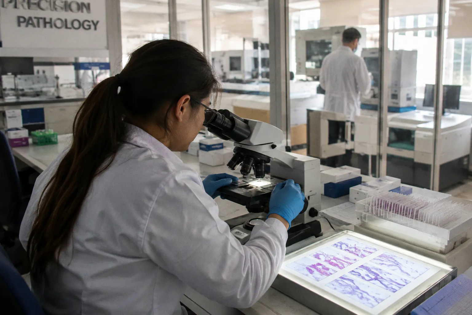
The computational pathology community solved this years ago by chopping the slide into patches, but that move creates a different bottleneck: how do you take tens of thousands of small tiles, each with weak signal, and turn them back into one clinically useful prediction? Attention-based Multiple Instance Learning is the answer the field settled on, and it's worth understanding exactly how it works before you trust the heatmaps showing up in your LIS.
A slide-level prediction is only as good as the aggregation step. Everything downstream — heatmaps, triage flags, sign-out decisions — lives or dies there.
From Gigapixel Raw Data to Instance Embeddings
The preprocessing pipeline is unglamorous, but it determines everything downstream. A scanner outputs a slide at 20x or 40x optical magnification. At 40x, you're working at roughly 0.25 micrometers per pixel. The file is then tiled into non-overlapping patches — usually 256×256 or 512×512 pixels — and each patch becomes an “instance” in MIL parlance. For a typical breast biopsy at 40x, you can easily exceed 50,000 patches per slide. For larger resection specimens or tissue microarrays, that number climbs further.
That patch count is not just a storage problem. It changes the statistical shape of the learning task. A conventional image classifier expects a single image, or a manageable batch of images, with a label attached to each one. A slide-level MIL system receives a bag containing many instances and usually only one label for the entire bag. Most of those instances may be benign, irrelevant, redundant, or technically compromised. The model therefore has to learn two things at once: what visual patterns are associated with the slide label, and which parts of the bag deserve attention in the first place.
Before any neural network touches the tissue, the staining has to be normalized. Hematoxylin and eosin look different depending on which lab processed the slide, which scanner acquired it, and how long the stains sat on the bench. The Macenko and Vahadane algorithms handle this by decomposing the RGB image into stain vectors and projecting to a canonical color space. Skip this step and your model learns lab signature instead of disease. Every vendor demo glosses over this; every production failure we've tracked traces back to it. Stain normalization isn't optional — it's the difference between a model that generalizes across sites and one that collapses the moment you move it from the development lab to a community hospital forty miles away.
Normalization is not a universal cure. It can also suppress visual information that is genuinely useful, especially when the target task depends on subtle differences in cytoplasmic or stromal appearance. The right question is not whether an algorithm makes slides look more alike. It is whether the transformation reduces unwanted technical variation without erasing morphology that the classifier needs. A robust pipeline should be assessed with external slides, not only with a before-and-after screenshot from the development set.
Background filtering is another silent prerequisite. Slides contain glass, pen marks, blur, fold artifacts, and regions where tissue simply isn't present. A tissue-detection mask — threshold-based, Otsu, or learned — removes these non-informative patches before the embedding step. Feeding thousands of blank or artifact tiles into the feature extractor wastes compute and contaminates the bag with noise that the aggregator has to absorb. It seems trivial. It isn't. Labs that skip background filtering consistently report noisier attention maps and degraded classification metrics, even when everything else in the pipeline is correct.
The mask also establishes a boundary around what the model is allowed to see. If tissue detection is too aggressive, small fragments, detached tumor nests, or pale regions of mucin can disappear before classification begins. If it is too permissive, folds and pen marks become legitimate candidates for attention. In a clinical system, those errors should be logged as preprocessing failures rather than blamed on the MIL model. A heatmap cannot recover tissue that was never included in the bag.
Then comes the feature extractor. A pretrained ResNet or pathology-specific encoder — CTransPath, UNI, Virchow — runs on each patch and outputs a fixed-length embedding, typically 768 to 1,536 dimensions. That embedding table, the “bag,” is what actually enters the MIL aggregator. Tile size matters. Magnification matters. Encoder matters. Get any of the three wrong and the rest of the pipeline is wasted compute. Foundation models trained on millions of pathology slides are now replacing ImageNet-pretrained backbones, and the improvement in downstream MIL performance is real — but only if the rest of the preprocessing chain holds up.
The embedding is a compressed description, not a diagnosis. Two tiles can be close in feature space because they share staining, texture, or tissue composition without being interchangeable for the clinical question. Conversely, tiles from the same biological process can be separated by blur, section quality, magnification, or a change in background. This is why the encoder should be treated as part of the model specification. Switching encoders while keeping the same attention head is not a cosmetic update; it changes the geometry of the bag and can alter which instances appear important.
There is also a practical distinction between offline and end-to-end pipelines. In many MIL implementations, embeddings are extracted once and stored, while the aggregator is trained over those fixed vectors. That approach is considerably cheaper and easier to reproduce. Other systems fine-tune the feature extractor using the slide-level loss, at least after an initial frozen-encoder stage. Fine-tuning may improve task-specific performance, but it also increases the risk that the encoder will absorb site-specific shortcuts. The more of the pipeline that is trainable, the more carefully the validation design has to separate slides, patients, institutions, and acquisition conditions.
Mechanics of Attention-Based Multiple Instance Learning
MIL is a weakly supervised framework. You don't get patch-level labels — only the final diagnosis for the slide. So the question becomes: given a bag of instances and one label, can the model figure out which instances actually matter?
Ilse and colleagues formalized the attention-based version of this in 2018. The core idea is elegant. For each instance embedding h_k, you compute a scalar attention score:
a_k = softmax(uᵀ · tanh(V · h_k))
where u and V are trainable weight vectors. The softmax ensures the weights sum to one across all tiles in the slide. The slide-level representation is then a weighted sum:
z = Σ a_k · h_k
followed by a classifier. The model learns which patches to attend to, and the attention scores themselves tell you which patches mattered. The permutation invariance is the key property — the bag-level prediction doesn't depend on the order you feed tiles in, which is exactly the behavior you need when the spatial arrangement of patches is arbitrary after tiling.
Permutation invariance is useful, but it comes with a trade-off. A plain ABMIL aggregator knows that an instance belongs to the same bag as the others. It does not automatically know where that instance sits on the slide, which tissue lies next to it, or whether several similar patches form a coherent architectural pattern. The weighted sum deliberately discards much of that arrangement. For tasks where the presence of a distinctive cellular pattern is enough, that may be a sensible simplification. For tasks involving invasion, gland formation, immune geography, or stromal organization, it can be a serious limitation.
Two practical variants emerged. The “gated” ABMIL adds a sigmoid gate that further sharpens the attention, giving the network more expressiveness in deciding which tiles carry signal and which are noise. CLAM — Clustering-constrained Attention Multiple Instance Learning — extended the framework by adding multiple attention branches, one per class, so the model can identify regions associated with different subtypes within a single slide. If you have a prostatectomy specimen with both Gleason 3 and Gleason 4 patterns, CLAM can in principle highlight each region independently. Both architectures produce interpretable heatmaps without needing pixel-level annotations. That's the whole trick. No expensive manual segmentation is required, but you still get back something a pathologist can look at on a Monday morning.
“In principle” is doing important work there. The attention branch is optimized to improve the bag-level objective, not to reproduce a pathologist's annotation. A high score means that the model used the instance strongly in forming its prediction. It does not prove that the tile contains the causal lesion, nor that every relevant tile received a high score. The distinction is easy to lose once the values are rendered as a persuasive red-to-blue overlay.
The training objective is straightforward: binary cross-entropy at the bag level. You backpropagate through the attention weights and, depending on the implementation, either keep the feature extractor fixed or fine-tune it using the same weak supervision signal. This is both the strength and the vulnerability of the approach — the model can learn powerful slide-level representations, but it can also overfit to spurious correlations if the dataset is small or the class distribution is skewed.
Class imbalance makes the problem particularly awkward. If positive slides are rare, the classifier can achieve a superficially attractive loss by learning a conservative decision boundary. If the positive class contains several visually different phenotypes, the attention module may settle on the easiest one and ignore the others. A pathologist may regard those morphologies as equivalent evidence; the model does not have that prior unless the training design supplies it through diverse examples, sampling, augmentation, or a suitable objective.
A useful evaluation therefore goes beyond slide-level AUC. It should examine sensitivity to site and scanner, calibration of predicted probabilities, stability of attended regions, and failure cases in which the prediction is correct for the wrong reason. If attention maps change dramatically when a few background tiles are removed, the model is not showing robust interpretability. It is showing a fragile dependency on the composition of the bag.
Overcoming Attention Concentration
Here is the friction point nobody talks about in vendor demos. Vanilla ABMIL tends to collapse. The attention concentrates on a tiny fraction of top-K tiles and effectively ignores the rest of the slide. This is a documented failure mode in the computational pathology literature. The model learns to identify a handful of “hero” patches — the most obviously malignant or most distinctive regions — and bets everything on them. The remaining tens of thousands of tiles receive negligible weight. It also creates a real overfitting risk: the model locks onto textural shortcuts in those few dominant patches and fails when the validation cohort comes from a different lab with different staining characteristics.
Why does this happen? The softmax normalization creates a winner-take-all dynamic. When a few patches produce unusually high activation in the attention network, the exponential in softmax amplifies the gap. Training reinforces this because the loss drops when those high-confidence patches are correct — even if the model is ignoring diagnostically relevant tissue elsewhere. In practice, this means your attention heatmap looks like a handful of red dots on an otherwise blue slide. Technically correct on the training set. Clinically unconvincing.
Concentration is not always a defect. If one small focus genuinely contains the decisive finding, a sparse map may be exactly what the model should produce. The problem is assuming that sparsity is automatically evidence of diagnostic precision. In a resection specimen, a convincing result may require a distributed pattern: multiple tumor foci, a relationship between tumor and stroma, or consistent morphology across sections of tissue. A model that focuses on one visually dramatic patch can achieve the right label while failing the underlying task.
ACMIL, introduced in 2024, attacked this directly. It uses Multiple Branch Attention (MBA) — separate attention heads with different random initializations — combined with Stochastic Top-K Instance Masking (STKIM). The masking step randomly drops high-attention patches during training, forcing the model to spread its bets across the slide. Each branch learns a slightly different attention distribution, and the ensemble of branches captures a more complete picture of diagnostically relevant tissue. The published benchmarks show more diverse attended regions and better generalization to external datasets.
The principle is broader than one architecture. Any method that prevents the aggregator from relying on a single dominant evidence source is trying to solve the same problem: make the model account for alternative instances and reduce the reward for shortcuts. Multiple branches, instance dropout, clustering constraints, diversity penalties, and top-K masking all change the pressure placed on the attention mechanism. None of them guarantees clinical validity. They simply make it harder for the easiest patch to win every time.
For clinical deployment, this matters more than any architecture benchmark. A model that lights up on three tiles and ignores the rest isn't trustworthy when the input distribution shifts. If your lab serves multiple hospital sites with different staining protocols and scanner models, the concentration problem will eventually bite you. The ACMIL fix is not a luxury refinement — it addresses a fundamental instability in vanilla attention pooling that surfaces under exactly the conditions production labs face every day.
| Architecture | Aggregation mechanism | Core contribution |
|---|---|---|
| ABMIL (2018) | Attention pooling | First trainable, permutation-invariant MIL aggregator |
| CLAM | Multi-branch attention | Class-specific attention heads and instance-level clustering |
| TransMIL (2021) | Self-attention with Nyström approximation | Long-range context across patch representations |
| ACMIL (2024) | Multiple Branch Attention plus STKIM | More distributed, deconfounded attention |
| MUSTANG (2023) | k-NN graph self-attention | Relationships among semantically similar patch embeddings |
The table is not a ranking. These models make different assumptions about what information is useful and how much structure can be recovered from weak labels. A simple ABMIL head can be the right choice when the encoder is strong, the task is relatively focused, and operational simplicity matters. A more elaborate model can be justified when the failure mode is clearly architectural rather than a consequence of poor tissue detection, label noise, or site shift.
Beyond Simple Pooling: Integrating Spatial Context and Graph-Based Attention
Pooling attention across instances treats the slide as a bag of unrelated patches. That works for some tasks. It fails when spatial structure matters — which is most of the time in histopathology. Tumor microenvironment isn't random. Lymphocyte infiltration patterns, gland architecture, stromal boundaries: these all depend on where tiles sit relative to each other. A cluster of tumor-infiltrating lymphocytes three tiles away from a gland means something different than those same lymphocytes scattered randomly across the slide. Bag-level MIL, by construction, cannot capture this.
The phrase “spatial structure” needs a little care. There are at least two different relationships a model might use:
- Physical neighborhood: patches are related because their coordinates place them next to one another on the slide.
- Semantic neighborhood: patches are related because their learned embeddings are similar, even if they are far apart in the tissue section.
Those relationships can overlap, but they are not interchangeable. Adjacent patches may contain a tissue boundary and therefore look very different. Distant patches may share the same morphology and belong to the same biological compartment. A graph built from coordinates captures the first relationship; a graph built from embedding similarity captures the second.
TransMIL, published in 2021, brought self-attention to the MIL setting. It uses Nyström approximation to make the quadratic cost of self-attention more tractable across large collections of patches. The result is that each tile's representation can be informed by other instances in the bag, rather than being reduced immediately to an independent scalar weight. This lets the model learn structural motifs — arrangements of tissue representations that carry diagnostic significance — without requiring a manual annotation for every spatial relation.
Coordinate handling is still a design decision. Some pipelines retain the original x-y positions and use them to arrange or encode patches before attention. Others reduce the slide to an unordered collection and rely on learned relationships among embeddings. The former preserves physical layout more directly but can be sensitive to tissue fragmentation and the coordinate system used by the scanner. The latter is more flexible about repeated morphology across a slide, but it should not be described as learning physical adjacency unless coordinates are explicitly part of the graph construction.
MUSTANG, introduced in 2023, took a different route. It constructs a k-nearest-neighbor graph in patch embedding space and runs graph-based self-attention over that graph. Each patch is connected to other patches that are close according to their learned feature representations. This captures semantic or embedding-space neighborhood relationships without paying the full cost of comparing every patch with every other patch. A neighbor in this graph may be located far away on the physical slide; the edge says that the two instances are similar in the representation space, not that they share a tissue boundary or sit next to one another.
That distinction is not a technical footnote. If a graph is built from embedding similarity, its edges may link morphologically similar glands, tumor regions, or stromal patterns distributed across the specimen. Such links can help the model identify repeated evidence. They cannot, by themselves, tell the model that one tile borders another. Physical adjacency would require slide coordinates or another explicit spatial construction.
MUSTANG's graph therefore offers a different kind of context from a coordinate-based neighborhood graph. It can connect distant but semantically related instances and reduce the number of pairwise relationships the model must process. It can also inherit the weaknesses of the encoder: if the embedding space groups patches by stain intensity or scanner artifact instead of morphology, the graph will faithfully propagate those errors. The graph is only as meaningful as the representation used to construct it.
In benchmark evaluations, MUSTANG pipelines have reported F1-scores around 0.89 and AUC up to 0.92 on weak-supervision classification tasks. Those are competitive numbers — and we should stress that benchmark performance and clinical performance are not the same thing. The choice of split, the number of institutions represented, the prevalence of the target finding, and the degree of patient-level separation all affect how those figures should be read. A graph model that performs well on a controlled dataset still needs external validation under the staining, scanning, and tissue heterogeneity of the intended service.
Both spatial and semantic graph approaches share a practical implication: tile metadata is no longer throwaway information. Coordinates, magnification, tissue masks, and embedding quality can all influence what the aggregator learns. If your vendor isn't feeding patch coordinates into a spatial model, ask why. If it claims to use graph attention, ask whether the edges represent physical proximity, embedding similarity, or both. The answer will tell you whether the system was built for publications or for patients.
Clinical Interpretability: Translating Heatmaps into Diagnostic Insights
The pitch from every vendor in this space is the same: the model highlights the malignant regions. That sentence is technically true and practically misleading.
What attention-based MIL actually produces is a tile-level importance map. You can color the slide from blue (low attention) to red (high attention) and overlay it on the H&E. CLAM-style architectures can do this per predicted class, so a multi-class model might show separate heatmaps for benign, low-grade, and high-grade regions. This is genuinely useful for sanity-checking the model — if the hot regions don't line up with what the pathologist sees, something is wrong. We use it that way routinely.
What it does not produce is a pixel-perfect tumor boundary. Attention weights are computed at the instance level, not pixel level. Each tile is 256 or 512 pixels wide. The attention score applies uniformly to that entire patch. Don't expect segmentation-grade masks. If you need that, you're in a different model class entirely — U-Net variants, SAM-style segmentors — and the vendor is overselling by conflating attention heatmaps with segmentation outputs.
The color scale can also mislead. “Red” usually means high relative attention within that slide or model output, not a calibrated probability that the tile contains tumor. A slide with no relevant lesion can still contain a relatively hottest patch. Conversely, a biologically important region may receive moderate attention because the classifier is using several supporting areas together. Heatmaps should therefore be read comparatively and alongside the original image, not as a standalone binary annotation.
Attention maps are most useful when they are tied to a defined workflow. A pathologist can use them to navigate a large slide, inspect the evidence behind an algorithmic flag, compare the model's focus with the morphology visible at higher magnification, and identify obvious failure modes. The map is less useful when it is displayed as decoration after the prediction has already been accepted. Interpretability has operational value only if a human can act on it.
There's also a regulatory gap worth naming. As of now, there are no standardized guidelines defining acceptable thresholds for attention heatmap reliance in clinical diagnostic reporting. The FDA has cleared several AI-assisted pathology products, but attention interpretability specifically isn't a regulated artifact. CE-IVD marking in Europe follows a similar pattern — the cleared device is the prediction, not the heatmap. Treat the heatmap as a second opinion, not a primary sign-out tool. A pathologist who overrides the heatmap based on their own read is doing exactly what the system is designed to support.
A workflow that holds up in production: the model triages the case, flags regions of interest, and the pathologist reviews both the slide and the heatmap before signing out. The model reduces friction on the easy cases and catches the ones a tired human might miss. That is the realistic value proposition — augmentation, not replacement. The labs that fail with these systems are the ones that deploy them as autonomous oracles instead of interactive decision support.
Interpretability should also be tested for stability. If the highest-attention tiles move whenever the slide is tiled with a slightly different offset, or if the map changes after a harmless compression step, the output needs to be treated cautiously. The same applies when a model highlights tissue outside the intended region of interest. A stable map does not prove that the model is correct, but an unstable map is a clear warning that the visual explanation is not ready to carry clinical weight.
The architecture is not the bottleneck. The bottleneck is the operational plumbing: scanner calibration, stain variability, pathologist workflow, LIS interoperability. Attention pooling solved the algorithm problem. The workflow problem is still yours.
Verdict
Is attention-based MIL ready for clinical deployment? Yes — with friction.
The 2018 ABMIL paper aged well. It's still the backbone of many production systems, and the attention-gated variant remains a sensible default for focused single-class problems. The advanced families — CLAM, TransMIL, ACMIL, MUSTANG — address real failure modes that surface the moment you deploy outside the training distribution. The preprocessing pipeline matters more than the architectural choice. A state-of-the-art aggregator on top of unnormalized stains and unfiltered backgrounds will produce garbage. And the heatmaps are useful, not infallible.
If you're a lab manager evaluating a vendor, ask four questions. Which MIL backbone are they running? Which encoder produced the embeddings? How do they handle stain normalization across your sites? Do they use any of the deconfounding techniques from ACMIL or similar work? If the sales engineer can't answer those, the deployment will fail in ways the demo won't show.
Add two more questions if the system claims to model context. Are graph edges based on physical slide coordinates, embedding similarity, or both? And how was the stability of the resulting heatmap assessed across scanners, tissue preparation conditions, and alternative tiling choices? A system that uses a semantic graph should not be sold as if it had learned physical adjacency. A system that produces an attention overlay should not be sold as if it had produced a segmentation mask.
Attention-based MIL didn't disrupt pathology. It didn't revolutionize anything. It gave us a workable way to turn gigapixel noise into a slide-level answer with a heatmap attached, and it survived contact with real clinical data. That's the verdict: deployed, useful, not magic.