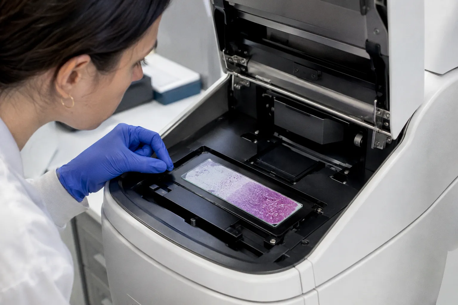
The operational failure is rarely visible in a dashboard. It appears as a silent batch effect: the tissue is biologically comparable, but its digital color signature is not.
For AI-assisted histopathology, that distinction is material. Deep learning models do not interpret slides in the abstract. They learn visual patterns from pixel distributions, tissue structures, and local contrasts. If one laboratory produces darker hematoxylin, another uses a warmer eosin tone, and a third operates a different optical scanner, the model may encounter a domain shift before it encounters the pathology.
Stain normalization in digital pathology is the computational response. It adjusts the appearance of digitized H&E slides toward a defined reference while attempting to preserve the biological structures that matter for diagnosis and image analysis. Used correctly, it can improve cross-site model performance. Used casually, it can introduce new artifacts, conceal process variation, and create a compliance problem disguised as an image-processing improvement.
The challenge of batch effects in multi-center histopathology
Physical staining is not a single controlled variable. It is a chain of variables.
The laboratory’s tissue processor, reagent lot, staining platform, timing, temperature, section thickness, and operator practice all influence the final H&E image. The scanner adds another layer through illumination, optics, camera response, focus behavior, and file-generation settings. Even when laboratories follow the same broad staining protocol, the resulting slides can differ in color intensity and balance.
For a human pathologist, many of these differences are manageable. Experienced readers routinely compensate for moderate shifts in hue and saturation. That does not mean the variation is operationally irrelevant. Human interpretation is contextual and adaptive. A machine-learning model is more dependent on the statistical distribution of its training data.
This creates a familiar pattern in computational pathology:
- A model performs strongly on internal validation data.
- Performance declines when slides come from another laboratory or scanner.
- The decline is attributed to the model architecture, even though the primary issue may be image-domain mismatch.
- Teams respond by collecting more data without first controlling the visual variability in the existing data.
- The development program becomes more expensive, slower, and harder to validate.
The financial exposure is straightforward. Every additional site, scanner, stain batch, and tissue type expands the validation surface. If the pipeline cannot distinguish biological signal from acquisition noise, the laboratory carries that uncertainty into deployment.
Stain variation is not merely a cosmetic defect. In an AI workflow, it is a data-governance and model-performance issue.
A multi-center dataset therefore requires more than sufficient case volume. It requires a controlled approach to image appearance. The objective is not to make every slide look identical for presentation purposes. The objective is to reduce irrelevant visual variation while retaining morphology, cellular architecture, and diagnostically meaningful features.
That distinction governs the entire design of a stain normalization pipeline.
Why standardization at the wet-lab level remains necessary
Computational normalization does not replace standardization of staining reagents or laboratory protocols. It sits downstream of them.
A laboratory that applies aggressive image normalization to compensate for unstable staining is not solving the root cause. It is moving the cost into software, validation, and maintenance. That may be acceptable as a short-term remediation strategy, but it is weak operational policy.
A defensible program has two controls:
1. Physical process control. The laboratory manages staining protocols, reagent supply, instrument maintenance, section quality, and scanner calibration.
2. Computational harmonization. The digital pathology pipeline reduces residual appearance differences that remain across sites and platforms.
This separation matters for compliance. If normalization is used to conceal an uncontrolled staining process, the laboratory may lose visibility into a change that should have triggered investigation. If it is used as a documented image-processing step after wet-lab controls are established, it becomes part of a traceable analytical workflow.
Statistical color transfer: from Reinhard to modern mapping
The earliest practical approaches to stain normalization treated the problem as a color-distribution mismatch. The premise is simple: if a source slide and a reference slide have different color statistics, transform the source so that its statistical profile resembles the target.
Reinhard normalization, published in 2001, is the clearest example. It maps the mean and standard deviation of pixel intensities from a source image to a reference image in the perceptual lαβ color space. The method does not require explicit separation of hematoxylin and eosin. It transfers global color statistics.
That simplicity is its main advantage. It is comparatively easy to implement, explain, and integrate into a whole-slide imaging workflow. It can be useful when the objective is broad appearance harmonization across a controlled dataset.
Its limitation is equally clear. H&E slides are not generic photographs. The two principal stains carry different structural information, and a global color transfer may not model their contributions independently. Tissue composition also varies across slides. A statistical mapping that performs acceptably on one organ type or staining range may behave differently on another.
For a production laboratory, the question is not whether a method is elegant. The question is whether its failure modes are visible, measurable, and acceptable for the intended use.
What a statistical transfer pipeline must control
A basic implementation often looks efficient because the mathematical operation is not conceptually complicated. The operational risk sits elsewhere—in reference selection, preprocessing, sampling, and quality assurance.
A robust pipeline should define:
- Reference slide policy. The target image must represent an approved staining appearance, not simply a convenient slide selected by an engineer.
- Tissue masking. Background, pen marks, empty glass, and non-tissue regions can distort color statistics.
- Sampling strategy. Whole-slide images are large. The pipeline must estimate parameters without allowing a small, unrepresentative region to dictate the transformation.
- Organ and stain scope. A reference suitable for one tissue type may not be appropriate for another.
- Output verification. Normalized slides must be checked for tissue structure, background behavior, artifacts, and downstream model impact.
- Version control. Changes to the reference image, transformation parameters, or software implementation require traceability.
The cost profile is also relevant. Whole-slide processing is a throughput problem. The pipeline must operate within the laboratory’s scanning, storage, and inference schedule. Research implementations frequently prioritize visual quality over processing economics. A clinical operation cannot.
Deconvolution strategies: Macenko and Vahadane frameworks
Color deconvolution methods address a more specific problem. Instead of treating the image as a single color distribution, they attempt to separate stain contributions and then reconstruct the image using a target stain appearance.
This approach is closer to the physical structure of H&E imaging. Hematoxylin and eosin contribute differently to the observed optical density. Estimating their stain vectors gives the normalization process a more meaningful representation of the slide.
The Macenko method
Macenko normalization, published in 2009, operates in optical density space. It uses singular value decomposition to estimate stain matrices and calculate maximum stain concentration vectors. The source slide can then be mapped toward a target template.
The method remains influential because it offers a practical balance between interpretability and computational utility. The pipeline has identifiable stages:
1. Convert image intensities into optical density values.
2. Exclude pixels that do not provide useful stain information.
3. Estimate the principal directions associated with stain appearance.
4. Calculate stain concentration information.
5. Reconstruct the image using the target stain characteristics.
This is not a trivial image filter. Each stage can affect the result. Threshold selection, tissue composition, background exclusion, and the target template all influence the transformation.
Macenko’s value is strongest when the laboratory needs a method that can be inspected and discussed in operational terms. The team can identify the stain matrix, review the reference template, and examine how the transformation behaves across representative cases. That does not eliminate validation. It makes validation more manageable.
There is also a performance consideration. Stain-vector estimation does not necessarily require exhaustive analysis of every pixel in a whole-slide image. Optimizing pixel sampling has been associated with execution speedups of up to 58 times in whole-slide processing engines. The exact benefit will depend on implementation, tissue distribution, hardware, and sampling strategy. The business point is more important than the headline: parameter estimation must be engineered separately from full-resolution image transformation.
The Vahadane method
Vahadane normalization, published in 2016, uses non-negative matrix factorization to separate stain appearance vectors from density maps. Its defining priority is structure preservation.
The method decomposes the image into components that represent stain appearance and concentration. The source slide’s appearance can then be adapted to a target while retaining the underlying density information associated with tissue structures.
That structure-preserving objective is operationally significant. Normalization that improves color similarity but damages nuclei, glands, stromal boundaries, or other relevant structures is not a successful normalization process. It is a visual transformation with clinical risk.
Vahadane can be useful where preserving morphology is a primary concern. It is also more demanding to evaluate. A laboratory must assess not only whether slides appear harmonized, but whether the normalization has altered edge definition, texture, cellular contrast, or the distribution of features used by downstream algorithms.
Macenko versus Vahadane
Neither method should be treated as a universal default. The appropriate choice depends on tissue type, scanner fleet, staining variation, downstream task, and available compute.
| Operational parameter | Macenko normalization | Vahadane normalization |
|---|---|---|
| Core approach | SVD-based estimation in optical density space | NMF-based separation of stain appearance and density |
| Main strength | Interpretable and practical stain-vector normalization | Strong emphasis on preserving tissue structure |
| Primary dependency | Quality of stain-vector estimation and target template | Stability of matrix factorization and decomposition |
| Typical deployment concern | Sensitivity to sampling, thresholds, and stain assumptions | Greater computational and validation complexity |
| Suitable evaluation focus | Cross-site color consistency and model performance | Structural fidelity, morphology preservation, and model performance |
| Management implication | Easier to standardize as a repeatable production step | Requires stronger review of image integrity and resource use |
The correct comparison is not which method produces the most attractive image. It is which method provides the best risk-adjusted performance for the intended use.
The target state is not visual uniformity. It is reliable morphology under controlled computational transformation.
Generative AI and image-to-image translation pipelines
Deep learning methods have expanded stain normalization beyond explicit color statistics and stain decomposition. Image-to-image translation models such as CycleGAN and Pix2Pix can learn mappings between image domains and generate a source image with the appearance of a target domain.
The attraction is obvious. These methods can capture complex relationships that are difficult to express through fixed statistical transfers or manually specified stain matrices. They may adapt to broader site-specific variation and do not necessarily require explicit stain deconvolution or optical density modeling.
The risk is also obvious. A generative model can alter more than stain appearance.
A production laboratory must assume that an image-to-image model may learn correlations that are not part of the intended transformation. It may change texture, local contrast, background behavior, or subtle structural features. A visually convincing result is not evidence of analytical safety.
Where generative normalization creates additional exposure
Generative pipelines expand the number of variables that must be controlled:
- Model architecture and training configuration.
- Source and target domain composition.
- Quality and representativeness of training slides.
- Cycle-consistency or reconstruction behavior.
- Handling of rare tissue structures and artifacts.
- Versioning of model weights.
- Monitoring for out-of-distribution inputs.
- Reproducibility across hardware and software environments.
- Review of changes after retraining or fine-tuning.
This is a governance burden, not just a technical one. A statistical transfer can often be explained as a defined transformation of image parameters. A generative model requires the laboratory to document training data, model behavior, performance boundaries, and change control with greater discipline.
For research applications, that complexity may be justified. For a clinical production environment, the expected operational gain must exceed the validation and maintenance cost. The burden should be demonstrated, not assumed away because the output appears smoother or more consistent.
CycleGAN and Pix2Pix are not interchangeable
CycleGAN is designed for unpaired image-to-image translation. This matters when the laboratory has slides from two domains but does not have matched images of the same tissue before and after normalization.
Pix2Pix typically relies on paired examples. Its use is therefore more dependent on the availability and quality of corresponding source-target image relationships.
The distinction affects deployment strategy. An institution with large, heterogeneous archives may be able to construct unpaired training domains more easily than paired datasets. That does not make an unpaired approach automatically safer. It changes the evidence required to prove that the model has learned stain appearance rather than site-specific biological or acquisition shortcuts.
A decision framework should include:
1. Define the intended transformation. State precisely what may change and what must remain invariant.
2. Separate training, validation, and deployment domains. Do not allow the same site or scanner distribution to dominate every stage.
3. Test rare and difficult cases. Normal tissue, necrosis, inflammation, low cellularity, folds, chatter, and staining artifacts may expose behavior hidden by average-case evaluation.
4. Review morphology independently of model scores. An improved AUC does not prove that tissue structure has been preserved.
5. Lock the model before clinical validation. Continuous retraining is incompatible with a stable validation claim unless the change process is formally controlled.
Building a wsi color standardization pipeline
Whole-slide image normalization is not an isolated preprocessing script. It is a production service connected to scanners, image management, computational infrastructure, AI inference, pathology review, and audit records.
The workflow should be designed around throughput and traceability from the beginning.
1. Establish the reference policy
A reference slide is not a decorative standard. It defines the target appearance against which source images are transformed.
The laboratory should document:
- Which tissue types the reference covers.
- Which scanner or image acquisition conditions produced it.
- How its staining quality was approved.
- Whether multiple references are required for different organs or workflows.
- How the reference is versioned and retired.
- Who has authority to approve a replacement.
A single reference for every tissue type may simplify administration while weakening performance. Conversely, a fragmented reference library can create uncontrolled complexity. The right level of segmentation depends on demonstrated variation and intended use.
2. Define the image-processing boundary
The pipeline must specify where normalization occurs and which downstream consumers receive the normalized output.
Potential destinations include:
- AI inference only.
- Pathologist review interfaces.
- Research image repositories.
- Training datasets.
- Telepathology services.
- Quality-control dashboards.
These uses are not equivalent. A normalized image used internally for model inference may require a different governance pathway from a normalized image displayed as part of the diagnostic record. The system must preserve the original image and clearly identify the transformed derivative.
3. Control compute and storage economics
Whole-slide images can be large, and normalization can create additional files, cache layers, and processing queues. A poorly designed pipeline increases storage consumption and creates a bottleneck between scanning and interpretation.
Management should track:
- Processing time by slide size and tissue content.
- Queue latency during peak scanning periods.
- CPU, GPU, and memory consumption.
- Temporary-file volume.
- Failure and retry rates.
- Cost per normalized slide.
- Impact on AI inference throughput.
A method that improves model metrics but doubles operational latency may be unacceptable for a high-volume service line. The business case must include the full workflow, not only the algorithmic result.
4. Preserve provenance
Every normalized slide should retain a machine-readable record of:
- Original image identifier.
- Source laboratory and scanner.
- Normalization method.
- Reference template or target domain.
- Software version.
- Parameter set.
- Processing timestamp.
- Success, warning, or failure status.
This is basic pathology informatics discipline. Without provenance, the organization cannot reproduce a result, investigate a discrepancy, or determine whether a model-performance shift followed a normalization change.
5. Create a failure policy
Normalization will encounter slides that should not be processed automatically. Examples include severe out-of-focus regions, excessive background, unusual stains, extensive tissue folds, unexpected color distributions, or images outside the validated domain.
The correct response is not to force every slide through the pipeline. A production system should be able to:
- Reject the slide.
- Route it for manual review.
- Return the original image for interpretation.
- Flag it for laboratory quality investigation.
- Record the exception without silently substituting a transformed output.
Automatic acceptance is not throughput. It is uncontrolled risk when the input is outside the model’s operating envelope.
Quantifying impact on AI generalizability and diagnostic accuracy
The central performance question is not whether the normalized slide looks more consistent. It is whether the transformation improves reliability without degrading clinically relevant information.
That requires evaluation at several levels.
Image-level assessment
Image review can identify obvious failures:
- Over-saturated nuclei.
- Washed-out eosin.
- Loss of contrast.
- Artificial background gradients.
- Halos around tissue structures.
- Texture changes.
- Reconstruction artifacts.
- Inconsistent appearance within a single slide.
Visual review remains useful, but it is insufficient. Human reviewers may accept an image that appears plausible while missing a subtle shift in the features used by an AI model.
Distribution-level assessment
The laboratory should compare source and normalized data distributions across sites, scanners, and batches. The objective is to determine whether irrelevant color variation has been reduced without collapsing meaningful biological differences.
This includes monitoring:
- Color channel distributions.
- Stain-vector behavior.
- Tissue-versus-background separation.
- Patch-level intensity patterns.
- Feature embeddings from the deployed model.
- Distribution shifts after scanner or reagent changes.
These measures are not substitutes for clinical validation. They explain why performance changes and help identify whether normalization is addressing the expected source of variation.
Model-level assessment
The most relevant evidence comes from external and multi-center testing. Internal validation often overstates performance because training and validation slides share acquisition characteristics.
The research indicates that effective color normalization can improve multi-center area under the ROC curve by up to 0.25 in some settings. That is a substantial potential gain, but it is not a guaranteed outcome for every tissue, task, or algorithm. The result depends on the quality of the normalization, the nature of the batch effect, the model, and the external dataset.
A separate result from the PatchCamelyon dataset showed that combining Macenko stain normalization with color data augmentation improved binary classification accuracy by 1.59% and F1 score by 2.50% over baseline. The operational lesson is not that Macenko should be deployed automatically. It is that normalization can work as part of a broader robustness strategy rather than as a standalone fix.
A serious evaluation program should compare at least four conditions:
| Evaluation condition | Purpose |
|---|---|
| Original images, original training pipeline | Establish the current baseline |
| Normalized images without other changes | Isolate the effect of stain normalization |
| Color augmentation without normalization | Measure the value of training-time robustness |
| Normalization plus augmentation | Test the combined production strategy |
The comparison should be performed across held-out sites, scanners, tissue types, and relevant patient or case strata. Average performance alone is not enough. The laboratory must inspect sensitivity, specificity, calibration, subgroup behavior, and failure patterns.
Diagnostic safety and human review
AI metrics do not replace pathologist oversight. A normalization method can improve classification performance while making a slide less comfortable or less transparent for human review. That trade-off must be addressed before deployment.
The evaluation should ask:
- Does the normalized image remain interpretable to the pathologist?
- Are diagnostically important structures preserved?
- Can the reviewer access the original image without friction?
- Is the normalized image clearly labeled?
- Does normalization alter the review time or disagreement rate?
- Are there tissue categories where the method should be disabled?
The answer may be task-specific. An algorithm used for triage, case prioritization, or quantitative scoring may tolerate a different normalization strategy from one used to support direct diagnostic interpretation.
Choosing between normalization approaches
Selection should be driven by the operating model, not by the popularity of a method in the literature.
A laboratory director or hospital administrator should require a written decision that covers:
- The source of observed variation.
- The clinical or operational task affected.
- The sites and scanners included in validation.
- The reference-slide strategy.
- The expected throughput.
- The computational budget.
- The audit and provenance design.
- The fallback path for invalid inputs.
- The evidence required for release.
- The change-control process after deployment.
For many organizations, a staged approach is more defensible than an immediate move to generative translation. Begin with a transparent statistical or deconvolution method. Establish the baseline. Measure external performance. Document failure modes. Only then assess whether a more complex model offers enough incremental value to justify its governance burden.
This is not conservatism for its own sake. It is margin protection. Every additional layer of technical complexity creates costs in validation, infrastructure, training, monitoring, and incident response.
A practical selection matrix
| Business and technical priority | More suitable starting point |
|---|---|
| Fast deployment with transparent parameters | Reinhard or another statistical color-transfer method |
| Explicit modeling of H&E stain components | Macenko-based normalization |
| Strong emphasis on structure preservation | Vahadane-based normalization |
| Large unpaired multi-site image domains | CycleGAN-style image translation, with extensive validation |
| Reliable paired source-target examples | Pix2Pix-style supervised translation |
| High-volume whole-slide processing | Method with optimized sampling, batching, and measured queue performance |
| Clinical deployment with strict traceability | Interpretable method with locked parameters and documented provenance |
The matrix is a starting point, not a release decision. No approach is universally optimal across every organ type or downstream task. Empirical validation remains mandatory.
Compliance, change control, and long-term maintenance
Normalization becomes part of the laboratory’s analytical environment as soon as it influences a clinical workflow or a validated AI model. That means it requires ownership.
The responsible organization should define who controls:
- Reference templates.
- Algorithm versions.
- Parameter changes.
- Scanner onboarding.
- New laboratory onboarding.
- Monitoring thresholds.
- Incident review.
- Revalidation triggers.
- Archival and rollback procedures.
A new scanner can change image distributions even when staining remains stable. A new reagent lot can change the stain profile even when the scanner is unchanged. A software update can alter normalization output without any visible change to the user interface. These events should be treated as potential sources of analytical drift.
Monitoring should therefore continue after deployment. The laboratory should watch for changes in normalized image distributions, model confidence, external-site performance, exception rates, and pathologist feedback. The objective is early detection, before the issue becomes a diagnostic incident or a costly retrospective review.
The original slide must remain available. A transformed derivative should never become the only record. The system should make it possible to compare original and normalized images, identify the exact processing path, and restore the prior pipeline if a defect is discovered.
That requirement has an economic benefit as well as a compliance benefit. Reconstructing thousands of cases after an undocumented image-processing change is expensive. Provenance is cheaper than remediation.
The operating position
Stain normalization in digital pathology is best understood as infrastructure. It is a control layer between slide acquisition and computational interpretation. Its value lies in reducing irrelevant variation, improving model portability, and making multi-center deployment more predictable.
The strongest programs will not advertise a single algorithm as a universal solution. They will define a controlled operating envelope. They will select a method that fits the tissue, task, scanner fleet, throughput target, and evidence standard. They will measure performance on external data. They will preserve original images. They will document every transformation.
The potential is meaningful. Multi-center AUC gains of up to 0.25 and measurable improvements in accuracy and F1 score demonstrate why the problem deserves attention. But the numbers do not remove the responsibility to validate. A normalization method that improves one benchmark can fail on another tissue type, another scanner, or another deployment environment.
The executive conclusion is simple: standardize the laboratory process first, then use computational normalization to manage the residual variation. Do not confuse a cleaner-looking slide with a safer analytical system.
Any organization deploying AI-assisted histopathology without a documented stain-normalization strategy, external validation plan, and rollback procedure is accepting avoidable operational risk. That is not innovation. It is an uncontrolled dependency in the diagnostic supply chain.